An ML platform I can actually run: 40,000 papers, six experiments, every layer underneath
At Cruise I worked on ML infrastructure for the autonomous vehicle trajectory ranking model: data generation pipelines and feature computation, at a scale where a single job could chew through petabytes. At Block I built observability systems for compliance screening, including an MCP server, written from scratch, that let engineers query production data in natural language to surface silent failures.
Those are two separate projects that touch ML application from different angles, and neither involved owning the platform underneath. At Cruise, the training orchestration and model registry and serving layer and monitoring were built and operated by other teams. I knew how to be a careful tenant of that system. I had never been the landlord.
So I built a small one, alone, end to end, trying to cover as many parts of a project like this as would fit in one repository. Semantic search over PubMed biomedical abstracts: ingestion, storage, embedding, evaluation, an API, monitoring, CI, a deployment I have to keep alive myself, and an MCP server so an AI assistant can use the whole thing as a tool.
That meant the modeling work as well as the plumbing around it. I built the evaluation harness first, then used it to run six experiments: comparing a general-purpose embedding model against a biomedical one, fine-tuning the embedder on PubMed text with contrastive learning, training a cross-encoder to re-rank results, distilling a larger domain model into a smaller one, training an embedder from scratch, and quantizing for inference. Two of those improved search substantially, one made it measurably worse, and all six have numbers attached.
I wanted both halves deliberately. Deciding whether to fine-tune or re-rank or quantize is an infrastructure decision as much as a modeling one, and you can’t make it well from either side alone: the training work is what tells you a change is worth 272 milliseconds of latency, and the serving work is what tells you the better model doesn’t fit in the memory you have.
It’s running right now, it costs nothing to operate, and you can either query it from this page or add it to your own assistant with one command.
- Try it here: the search box below, or pubmed-search-683d.onrender.com/docs
- Give it to your AI assistant:
claude mcp add --transport http pubmed https://pubmed-search-683d.onrender.com/mcpand it can search 40,000 papers mid-conversation (details) - Code: github.com/chibanaryan/pubmed-ml-platform
- Serving model: huggingface.co/chibanaryan/minilm-pubmed-onnx
It’s a long post, so here’s the shape of it. How the pieces fit together follows one paper through the whole pipeline, from scheduled ingestion into Postgres and pgvector, through the embedding pipeline and experiment tracking, to the async serving layer, and names what each design choice cost. Measuring quality without labels is the evaluation harness, and six experiments is the training work it made possible: contrastive fine-tuning, cross-encoder re-ranking, knowledge distillation, and quantization, negative results included. When the hosting died is how a quantization experiment became the production serving path in order to survive a 512MB budget. Using it from your own assistant is the MCP server. Operating it is the parts that make it a system rather than a demo: a CI gate on model quality, A/B routing, metrics and alerting, load testing.
What semantic search is, briefly
Keyword search is string matching. You search “creatine muscle” and get documents containing those characters. It fails the moment someone phrases a question differently than the document is worded.
Semantic search converts text into vectors instead. Run a sentence through an embedding model and it outputs a few hundred numbers representing that sentence’s meaning as a point in high-dimensional space. “Creatine helps with muscle recovery” and “supplementing with creatine after resistance training aids repair” land near each other, despite sharing almost no words.
To search, you embed the query the same way and find the stored vectors closest to it, where “closest” means cosine similarity: are these two vectors pointing in roughly the same direction? Type a question, get back papers about that concept regardless of exact wording.
That’s the ML part, and it’s the small part. Everything else is infrastructure.
Try it
The corpus is 39,731 PubMed abstracts across nutrition, exercise physiology, psychology, behavioral science, and bioethics.
Try: gut microbiome and mental health · effects of meditation on anxiety · resistance training for older adults
Same thing from a terminal:
curl -X POST https://pubmed-search-683d.onrender.com/search \
  -H "Content-Type: application/json" \
  -d '{"query": "does creatine help with muscle recovery", "top_k": 3}'
1. "Short-term creatine supplementation enhances strength, reduces fatigue,
and accelerates recovery in resistance-trained athletes: a double-blind,
randomized, crossover trial." (0.677)
Journal of the International Society of Sports Nutrition, 2025
2. "Creatine monohydrate supplementation for older adults and clinical
populations." (0.659)
Journal of the International Society of Sports Nutrition, 2025
3. "Effects of creatine supplementation on muscle strength gains: a
meta-analysis and systematic review." (0.658)
PeerJ, 2025None of those titles contain the word “help.” That’s the point.
The more fun way to use it is to hand it to an AI assistant instead of reading results yourself. One command adds this corpus as a tool your assistant can call mid-conversation, so it can search, follow up on what it finds, and answer with paper IDs you can check. That’s further down, and it’s the part I use most.
How the pieces fit together
This is the part I most wanted to learn, so it gets the most space. Here is every component and the job it does.
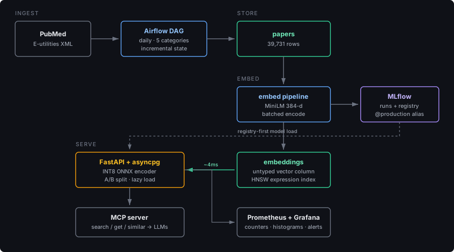
Follow one paper through the system.
Stage 1: A paper arrives (Airflow)
Airflow is a scheduler for data pipelines. You define a workflow as a graph of tasks, and it runs them on a schedule, retries the ones that fail, and remembers what already succeeded. Mine runs daily: five tasks that fetch new papers per subject area, load them, embed them, and report what happened.
Each run asks PubMed’s E-utilities API, an XML service from an older era of the web, for papers published since the last successful run in each of five subject areas. Those areas are defined by MeSH (Medical Subject Headings), the taxonomy the National Library of Medicine uses to tag every paper it indexes. Real human indexers read each paper and assign terms like “Creatine” or “Resistance Training.” That tagging becomes important later, because it’s the only ground truth I have.
The “since the last successful run” part is the piece worth dwelling on. The DAG keeps a cursor per subject area in its own database table, so a restart doesn’t refetch three years of papers, and a failed run resumes instead of starting over. That bookkeeping is most of what an ingestion pipeline actually is.
Two things this stage taught me.
First, orchestrators generate load, and a client’s own politeness doesn’t survive being run in parallel. The client throttles itself to the documented three requests per second, but that throttle lives inside one instance, so five concurrent category tasks each rate-limited themselves correctly and collectively hit the API at five times the allowed rate. The fix belongs in the orchestrator, which is the only thing that knows how many copies are running: fetches are now bounded to one at a time, with backoff for the 429s that still arrive.
Second, bad data enters here and never announces itself. While writing this post I checked a paper the system had stored and found its title was the fragment “The Impact of ” and nothing else. PubMed italicizes species names inside titles, and my XML parser used a method that returns only the text preceding the first nested tag. Every title containing an italicized organism or a subscripted chemical formula was silently cut off at that point, about 1% of the corpus. The abstract parser three lines below it in the same function handled this correctly. Ingestion is where quality problems are cheapest to prevent and most expensive to discover.
Airflow is honestly overkill at this scale. A cron job would move the same data. I used it because owning the orchestration layer, rather than being handed one, was the thing I wanted practice with.
The first run for a subject area backfills years of history, capped at the ten thousand records PubMed will page through for any one query, and the rest arrives over following days. After that a daily run is small: on a recent one, a category already caught up ingested eleven new papers.
Stage 2: Where it lives (Postgres and pgvector)
Papers land in Postgres. Their vectors land in the same Postgres, in a second table, using pgvector, an extension that adds a vector column type and distance operators to a normal relational database.
The alternative is a dedicated vector database like Pinecone or Weaviate. I chose against it. At this scale a specialized store buys speed I don’t need while adding a second system to keep in sync with the first: every paper would exist in two places, and every ingestion would need to succeed twice. Keeping vectors beside the metadata means a search result comes back with its title, journal, and MeSH terms in a single query, with no join across a network.
One decision here shaped everything downstream. I wanted to compare two embedding models, and they produce different-sized vectors: MiniLM gives 384 numbers per paper, PubMedBERT gives 768. If I declare the column as holding 384-dimensional vectors, the other model’s output is rejected on insert. So I left the column’s dimension unspecified and added a model_name column to distinguish rows.
That bought me clean model comparisons and cost me safety, in a way that took me a long time to see.
One smaller thing I got wrong first: Airflow needs its own database for scheduling bookkeeping, and I originally pointed it at the application database. It created about fifty metadata tables of its own alongside my three, which works fine and makes the schema unreadable. It now runs against a separate Postgres instance. Orchestration state and application data have no reason to share a home.
Stage 3: Text becomes vectors (the embedding pipeline and MLflow)
A pipeline reads papers that don’t yet have a vector for a given model, encodes them in batches, and writes the results back. It runs as the DAG’s final task, and also as a standalone command when I want to embed a specific model on demand. Three properties are what make it safe to schedule rather than merely automatic:
- Idempotent and resumable. It selects papers by the absence of a vector, so re-running costs nothing and a crash halfway through loses nothing. There’s no cursor to corrupt and no “which rows did I already do” bookkeeping.
- Capped per run. It embeds at most 5,000 papers at a time, so one run has a bounded duration. A backlog drains over consecutive runs instead of producing a single job that runs for an hour and fails at minute fifty-nine.
- Aware of its storage budget. It checks database size before writing and stops when over a configured limit, because the hosting plan has a hard ceiling and a database that fills up mid-write is worse than one that stops early. The limit is configuration rather than a constant, since a quota belongs to the hosting plan and not to the pipeline.
The models in this project are built and run with PyTorch, the standard framework for neural networks. It’s capable and it’s heavy: installed with its wrapper libraries, it runs well over a gigabyte. But running a finished model needs far less machinery than training one, so this task skips PyTorch entirely. It encodes with a compact copy of the model in a portable format called ONNX, the same encoder the production API uses. That keeps a gigabyte-plus dependency out of the scheduler rather than installing it there only to compute vectors the API can already produce, and it makes documents and queries pass through identical weights.
The trade is that this compact model is a hair less accurate than the full-precision original. But the production API already accepted that trade, for reasons that get their own section later, so matching it here costs nothing extra. Ranking quality on the resulting corpus, where some vectors came from the older full-precision model and some from the compact one, measures 0.8267 NDCG@5 against the 0.83 baseline. The two coexist without a meaningful penalty.
Every run is logged to MLflow, which is a system of record for machine learning experiments: parameters in, metrics out, model artifacts stored and versioned. Without something like it you end up with a directory of model files named final_v2_actually_final and no memory of which produced which number. With it, every claim in the experiments section below has a run behind it.
MLflow also acts as a registry, meaning models get versions and labels. Tag a version @production and the API loads that one on next start. Swapping the live model becomes an operation rather than a code change and a deploy.
Stage 4: Making search fast (HNSW indexes)
Comparing a query against 40,000 vectors one at a time works but is slow. An HNSW index builds a navigable graph of the vectors so search visits a small fraction of them, trading a little accuracy for a lot of speed.
Here is where the untyped column from Stage 2 sends its bill. pgvector can’t index a column whose dimension it doesn’t know. The workaround is an index on a cast expression:
CREATE INDEX idx_embeddings_hnsw_384
    ON embeddings USING hnsw ((embedding::vector(384)) vector_cosine_ops);
And from then on, every query has to cast both sides the same way, or the planner ignores the index:
ORDER BY e.embedding::vector(384) <=> $1::vector(384)Miss a cast and nothing breaks. No error, no warning. The database quietly compares your query against every row: roughly 80ms instead of 4ms, a 20x regression visible only if you measure. I spent more time working out why my queries weren’t using the index than I spent writing the entire serving layer.
It’s worth being precise about what that decision actually cost, because it isn’t the 80ms.
A typed column makes the rule impossible to break: declare vector(384) and Postgres rejects anything else, no discipline required. Leaving the dimension off moved that rule out of the database and into my head, where it holds only as long as everyone writing queries happens to know about it. And it fails quietly. A missing cast doesn’t error, it returns perfectly correct results, slowly.
For a solo project whose entire purpose was comparing models, I’d take that deal again. On a team it’s a bad one: someone adds a query six months from now, never having heard about the cast, sees correct results in review, and ships a 20x slowdown that surfaces whenever somebody finally profiles it. Schema constraints are how you make knowledge outlive the person who has it.
Stage 5: A query arrives (FastAPI and asyncpg)
FastAPI handles HTTP. When a search comes in, it encodes the query text into a vector with the same model used on the documents, then asks Postgres for the nearest stored vectors.
Talking to the database is asyncpg, a driver built for asynchronous Python. The distinction matters more than it sounds: with a synchronous driver, the process sits idle during every database round trip and can’t serve anyone else. With an async driver and a connection pool, the server handles other requests while Postgres is working. Same hardware, considerably more throughput.
The model itself loads lazily, on first request rather than at startup, and stays cached in memory afterward. That keeps deploys fast and means a restarted server is answering health checks in seconds instead of waiting to load weights.
Stage 6: Who’s asking
Three kinds of client hit that API. A browser, like the search box above. An MCP server, which exposes the same endpoints as tools an AI assistant can call, covered below. And Prometheus, which scrapes a metrics endpoint every 15 seconds and stores the counts and latencies over time, with Grafana drawing them.
The decisions, collected
| Decision | Why | What it costs |
|---|---|---|
| pgvector, not a dedicated vector DB | One system to operate; results and metadata come back together | Fewer vector-native features; would revisit past ~1M vectors |
| One untyped vector column for two models | Clean apples-to-apples model comparison in one table | No dimension safety; every query needs a cast or it silently scans everything |
| MeSH terms as relevance labels | Quantitative evaluation with no annotation budget | Measures topical overlap, not whether the paper answers the question |
| Airflow for a job cron could run | Practice owning orchestration: state, retries, parallelism | Real operational weight for a five-task pipeline |
| asyncpg over psycopg2 | Non-blocking DB calls, higher throughput per instance | Different parameter syntax, and a driver-level bug I’ll get to |
| INT8 quantized model in production | Fits in 512MB of RAM, encodes 5x faster | Slightly worse ranking quality, quantified below |
Measuring quality without labels
You can’t improve what you can’t measure, and measuring search quality normally means paying humans to rate results. Not happening for a side project.
MeSH terms are a usable substitute. If I search “creatine supplementation and muscle recovery” and the top results carry the tags “Creatine” and “Dietary Supplements,” the search is probably working.
So I built an evaluation harness: 8 queries across all five subject areas, each declaring which MeSH terms indicate high, medium, or low relevance. A paper matching two high-relevance terms scores 3, one high plus a medium scores 2, on down to 0. Then I compute NDCG, a ranking metric that rewards putting the best results at the top rather than merely including them somewhere in the list. A perfect ranking scores 1.0. The @5 in “NDCG@5” means it only grades the first five results, which is roughly what a person actually looks at.
Baseline MiniLM over 39,731 papers: 0.83 NDCG@5, 0.91 NDCG@10, mean search latency 3.9ms.
This is not a substitute for real annotations, and I’d distrust it for fine-grained comparisons. But it’s automatic and reproducible, and it turned every later decision into a measurement instead of an argument. Building the ruler before doing the work is the habit I’d carry to any project.
Six experiments
Up to here, the search engine used an embedding model exactly as its authors shipped it. But that model isn’t fixed. It’s a neural network, which for our purposes is a very large grid of numbers, and those numbers got their values through training: showing the model example after example and nudging the numbers each time until its output improved. Since training is just adjusting those numbers, I could adjust them further.
That opens up a menu. I could keep training the model on biomedical text so it understood the domain better, which is called fine-tuning. I could add a second, slower model that re-examines only the top handful of results. I could try a bigger model built for medicine, or shrink my model so it runs cheaper. Six experiments, aimed at two different goals: make the ranking more accurate, or make serving it cheaper. Each was measured against the same 0.83 baseline, with the same harness, so the numbers are comparable.
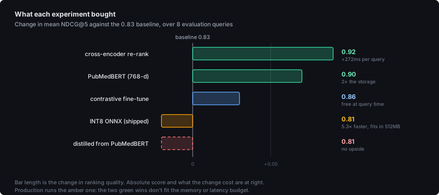
Cross-encoder re-ranking: 0.83 → 0.92. This is the “add a second model” idea, and it works because of a limitation in the first one. To make search fast, the embedding model turns each paper into a vector ahead of time and never looks at it again; at query time it only compares vectors, so the query and the document never actually meet. A different kind of model, a cross-encoder, reads a query and a document together and scores how well they match, which lets it notice that a paper mentions HIIT once in passing rather than being a whole study about it. The catch is that there’s nothing to precompute: it has to read every document fresh against each query, which is hopeless across forty thousand of them.
The standard resolution is two stages. The fast model retrieves 50 candidates, the slow model reorders those 50. I trained the re-ranker on about 20,000 (query, document, score) triples built from MeSH overlap, with graded targets rather than binary ones, so it learned degrees of relevance instead of a yes/no. The effect concentrates exactly where you’d hope: the HIIT query, worst in the corpus at 0.59, went to a perfect 1.00. Cost is about 272ms per query, the largest quality gain of anything I tried and by far the most expensive.
Contrastive fine-tuning: 0.83 → 0.86. This is the fine-tuning from the menu above: the default model was trained on general English and had never seen biomedical text, so I kept training it on mine. To teach a model that two things are related, you show it pairs of things that belong together, and MeSH hands those over free: two papers tagged with at least two of the same meaningful terms are probably about the same subject. Filtering out tags that say nothing topical, like “Humans” and “Retrospective Studies,” left roughly 100,000 such pairs.
The training trick here is elegant enough to be worth a sentence. You never have to supply counter-examples of things that don’t go together, because within each batch of pairs, every other paper is already a counter-example: nudge each true pair closer, push everything else in the batch apart. One pass over the data, 20 minutes on my laptop’s GPU.
The gains landed almost entirely on the previously weakest queries, sleep deprivation and HIIT, while the strong ones held. Lifting the floor without lowering the ceiling is the best shape this kind of result can take. It also carried an infrastructure cost that a pure modeling view would miss: a fine-tuned model produces different vectors, so evaluating it honestly meant re-embedding all 40,000 papers and storing them under a separate model name to compare like with like.
Swapping in PubMedBERT: 0.83 → 0.90, eventually. Early on, at about 10,000 papers, the general-purpose model beat the biomedical specialist on my metrics, so I shipped the generalist and moved on. Later I re-ran the comparison at full corpus size:
| Query | MiniLM | PubMedBERT |
|---|---|---|
| Creatine + muscle recovery | 1.00 | 1.00 |
| Psychological effects of quitting alcohol | 0.59 | 0.65 |
| HIIT benefits | 0.59 | 0.89 |
| Vegetarian protein | 0.97 | 0.88 |
| AI ethics in healthcare | 0.92 | 1.00 |
| Sleep deprivation + cognition | 0.67 | 0.81 |
| Gut microbiome + mental health | 0.87 | 0.95 |
| Resistance training for elderly | 1.00 | 1.00 |
| Mean NDCG@5 | 0.83 | 0.90 |
The specialist wins 5 of 8 and ties 2. At 10,000 papers the corpus was too sparse for domain knowledge to matter; at 40,000 there were enough near-miss documents for it to sort correctly. A benchmark conclusion is only valid at the scale you measured it. I had made a production decision on a number that didn’t survive more data.
That table is also the clearest picture of what the evaluation harness produces. The weak queries are weak for a legible reason: the corpus holds fewer papers tagged for “HIIT benefits” than for creatine, so there’s less available to rank correctly.
Knowledge distillation: 0.83 → 0.81. Distillation means training a small, fast model to imitate a big, slow one, the idea being that you keep most of the quality at a fraction of the cost. I trained my small model to reproduce the biomedical model’s sense of which papers resemble each other. It helped on two queries and hurt three, netting a small loss. The reason is instructive: “which papers look alike” is not the same as “which papers should rank above which,” and only the second one is what search needs. Fine-tuning won because its MeSH pairs described the actual task, and distillation only copied a general impression.
Training from scratch: no result. Fine-tuning starts from a model that already works. Here I did the harder thing, building an embedding model up from a raw, untrained language model. The training ran fine, but I could never score it: its vectors were twice the size of my existing ones, and 40,000 of them wouldn’t fit alongside what was already in the database within the free tier’s 512MB, which had no room to spare and doesn’t reclaim deleted space quickly. A storage quota ended a modeling experiment, which is a kind of wall I’d never personally hit before.
Quantization: 5.3x faster, 0.017 quality lost. This is where the compact model from Stage 3 came from. I exported the trained model to ONNX, the PyTorch-free format from earlier, then quantized it to INT8: weights stored as 8-bit integers instead of 32-bit floats, roughly a quarter the size, some precision discarded. Encoding went from 4.41ms to 0.84ms. At the time I filed this under interesting-but-unnecessary, since the database was my bottleneck, not the model.
Four months later it saved the project.
When the hosting died
I originally deployed to Fly.io. The trial ended, the app suspended itself, and reviving it required a credit card. Hugging Face Spaces was my fallback until I discovered they had made Docker Spaces a paid feature. I wanted this running and publicly queryable for free and indefinitely, because a portfolio project behind a dead link is worth nothing.
What remained was Render’s free tier: 512MB of RAM and a tenth of a CPU core.
PyTorch and its sentence-transformers wrapper need roughly 1.5GB resident just to encode one query. No configuration of the existing system fit.
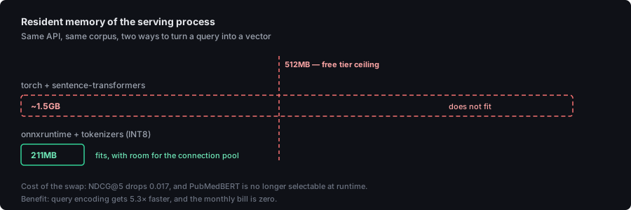
But the quantized ONNX model was still sitting in a directory from the experiment I’d dismissed, and ONNX Runtime doesn’t need PyTorch at all. If I could encode queries without importing torch, the whole stack would collapse.
So I wrote a second serving path, chosen by an environment variable, that loads the quantized model with ONNX Runtime and the tokenizer with a standalone library. The catch is that the step converting per-token vectors into one sentence vector isn’t part of the exported model, so I reimplemented it in about six lines of numpy. Model files live on the Hugging Face Hub and download on first request, keeping the container small.
Measured in a clean environment: 211MB against a 512MB ceiling. Compute on Render, database on Neon, model artifacts on Hugging Face, $0/month.
Then searches took 1 to 2.2 seconds, against 70ms on my laptop.
I found it without a profiler, using the other endpoints as instruments. Fetching a paper by ID, which only touches the database, took about 100ms. Finding similar papers, which does a vector search but no encoding, took 65ms. Both fast, so the database was innocent and encoding was the suspect. ONNX Runtime sizes its thread pool to the number of visible CPUs, but the container gets a tenth of one core, so those threads spent their lives fighting each other for a sliver of CPU. Pinning it to a single thread brought warm searches to 75–99ms, with per-stage logging now showing encode at 30–60ms and the database at 37–50ms.
The honest summary of this whole episode: production serves a model scoring 0.81 when 0.90 was available, because 0.90 doesn’t fit in the budget. Being able to state that tradeoff precisely, in ranking points against megabytes, is the entire skill. The quality ceiling of a deployed system isn’t set by the best model you can train. It’s set by the best model you can afford to serve.
Using it from your own assistant
The Model Context Protocol is a standard way for AI assistants to call external tools. Rather than build a chat interface nobody asked for, I exposed the search API as three MCP tools (search_papers, get_paper, find_similar) so any assistant that speaks the protocol can use this corpus.
This is the part of the project I had the most prior footing on. The MCP server I built at Block let engineers ask questions of production data in natural language and get grounded answers, instead of hand-writing queries against systems they only half remembered. The subject matter has nothing in common with biomedical abstracts, but the shape of the problem does: there’s a corpus somebody wants to reason about, and the bottleneck isn’t the model’s intelligence, it’s whether the model can reach the data.
It’s hosted, so there’s nothing to clone. In Claude Code:
claude mcp add --transport http pubmed https://pubmed-search-683d.onrender.com/mcpOr in any client that takes JSON config:
{
  "mcpServers": {
    "pubmed": {
      "type": "http",
      "url": "https://pubmed-search-683d.onrender.com/mcp"
    }
  }
}
The three tools it exposes are search_papers, get_paper, and find_similar.
Opening that URL in a browser won’t show you a search engine, incidentally. The protocol requires clients to declare they accept a streaming content type, and a browser doesn’t, so early visitors got a raw protocol error. The endpoint now detects browsers and serves setup instructions instead, which is a small thing but the kind of small thing that decides whether someone tries your project or closes the tab.
Two implementation notes, both consequences of the free tier. The transport is stateless, meaning each request stands alone: the server sleeps after fifteen minutes idle, and a session identifier outliving the process would only produce confusing errors. And it runs inside the existing API process rather than separately, so the tools reach the search endpoints over loopback instead of leaving for the public internet and coming back. Adding it cost no measurable memory, since the protocol library reuses machinery the web framework already loads.
Testing it is worth a note too, since a tool server that only works when a live API is up is a testing problem. The test suite swaps in a mock HTTP transport, so the MCP layer’s formatting, argument handling, and error paths are all exercised in CI with no network and no database.
Here’s an actual exchange, where the assistant decides on its own to call the tool, reads what comes back, and answers with IDs I can check:
Me: What does the recent literature say about gut microbiome
    and anxiety? Any promising interventions?

Claude: [calls search_papers: "gut microbiome interventions
         for anxiety", top_k: 10]

    The gut-brain axis is a bidirectional communication network
    linking gut microbiota to the CNS via neural, endocrine, and
    immune pathways. Dysbiosis is consistently associated with
    anxiety and depression across multiple reviews.

    Promising interventions:

    Probiotics — A 2025 pilot RCT (PMID 41097163) showed
    Weizmannia coagulans BC99 improved anxiety scores, working
    through the gut microbiota-brain axis.

    Prebiotics — An RCT by Johnstone & Cohen Kadosh (PMID
    40532960) tested 28 days of galacto-oligosaccharide
    supplementation in 83 young women, targeting trait anxiety.

    Diet — Mediterranean-style diets and reduced ultra-processed
    food intake show the most consistent links to lower anxiety.

    The field is moving from observational to interventional
    evidence, though most RCTs are still small.
Every claim carries an ID I can verify against the source. This is the piece I actually use.
Operating it
The rest is the unglamorous work separating a demo from a system.
A model quality gate in CI. Every push runs linting, type checking, and 50 tests with coverage, then builds and pushes a container image. Separately, because it needs a populated database that CI doesn’t have, an on-demand job runs the full NDCG evaluation against production data and fails if the mean drops below 0.80. Last run: 0.8275, passed. Ordinary CI catches code regressions. This catches model regressions, which are the ones that ship quietly.
A/B routing. Two environment variables send a configurable share of traffic to a second model. Every response reports which model served it, and request counts and latencies are tracked per model, so a comparison can run against real traffic instead of my eight evaluation queries.
Monitoring that actually counts. My first version was a hand-rolled dictionary of counters. It exposed an error counter that was incremented in exactly zero places, and had therefore reported a reassuring 0 since the day I wrote it. I replaced it with the standard Prometheus client: counters and latency histograms with proper labels, incremented in middleware that sees every request and every exception. Histograms rather than averages, because you cannot recover a 95th percentile from a mean. Then alert rules for the three conditions worth waking up for: service down, error rate above 5%, p95 latency above 500ms.
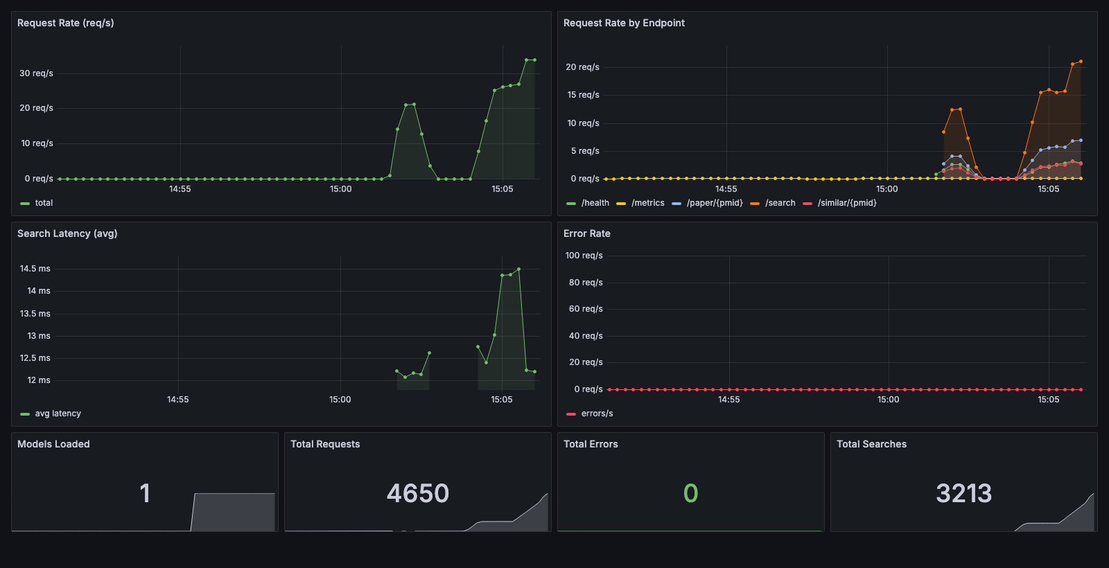
That’s the local stack under load-test traffic. The two humps are Locust runs. The per-endpoint panel is the labeled metrics paying off: /search, /paper/{pmid}, /similar/{pmid}, and /health are separable, so a latency problem can be attributed to a route instead of averaged into fog.
Being straight about the boundary: Prometheus and Grafana run in the local Docker Compose stack, not in production. The deployed API exposes its metrics endpoint, but nothing on the free tier scrapes it, because a scraper and a time-series database don’t fit in what’s left of 512MB. Monitoring is the first thing I’d add back with a real budget.
Setting this up taught the same lesson twice. When I checked the panels against live data, the error rate panel read “No data” rather than 0, because a counter with no recorded errors emits no series at all. Visually, a healthy service and a broken metric looked identical, which is precisely the failure I had just spent an afternoon fixing one layer down. The panel now falls back to zero explicitly. An uninstrumented counter is worse than no counter, and a panel that can’t distinguish “fine” from “missing” is worse than no panel.
A test suite that needs nothing installed. 50 tests covering the ingestion client’s XML parsing, the ranking math, the API endpoints, the embedding pipeline, the model registry, and the MCP layer. None of them need Docker, a database, or a downloaded model: the connection pool is mocked, the embedding model is patched out, and the MCP tools run against a fake HTTP transport. The whole suite finishes in about five seconds, which is what makes it something I actually run rather than something CI runs at me. The tradeoff is the one described above, and it’s a real one: a suite this isolated cannot see a driver-level contract break.
Containers that don’t ship build tools. A multi-stage Docker build compiles dependencies in one image and copies only the installed packages into a slim runtime image, so compilers never reach production. Installing PyTorch from its CPU-only index rather than the default took the image from 3.5GB to 641MB, since the default build drags in a full CUDA toolchain for a GPU that no deployment target here has.
Load testing. 20 concurrent users for 60 seconds: 2,019 requests, zero failures, 34 requests per second. Half of those finished in under 15ms, 95% within 71ms, and 99% within 460ms. That last number is the interesting one, because averages hide it: a small fraction of requests are far slower than typical, and here the cause is every user sharing a single in-process encoder. It’s the clearest argument for moving query encoding into its own service.
What broke
Two failures generalize past this project.
A broken feature that nothing in the system could have told me about. When I moved from the synchronous database driver to the async one, all 28 tests passed, so I deployed and went on to other things. Months later, running a live query before writing this post, the first search returned a 500. asyncpg has no encoder for pgvector’s type: passing a Python list raises a type error, and the value has to be serialized to a specific text format first. The old driver had quietly tolerated the list.
The tests missed it because they mock the database connection. A mocked query happily accepts a list, returns fixture rows, and asserts the response shape is correct. Every assertion was true and the feature was dead.
The part worth sitting with is that three separate safety nets had the same hole. The tests never touched a real database. The error counter that should have spiked was, during exactly this period, the one incremented in zero places. And nobody was using the thing yet, so no traffic existed to trip either. Any one of those working would have caught it the day I shipped it, and I had built all three.
Mocks verify the shape of a conversation, not that the other party understood you. The fix was one line; the lesson was that a test suite mocking the boundary it most needs to check is a suite that passes for the wrong reason.
A fix that looked wrong because it never shipped. The single-thread change described earlier didn’t appear to work: I pushed it, measured, and saw no improvement. The fix was correct. It had never deployed. Services created through Render’s API from a public repository don’t get a webhook, so auto-deploy silently does nothing, and the server was still running my first build. Before concluding a fix didn’t work, confirm the thing you’re testing contains it.
What I’d do differently
Query encoding shares a process with request serving. It belongs in its own service, so it can scale on different hardware and stop poisoning tail latency.
The MeSH proxy was good enough to choose a model and measure fine-tuning gains, but 50 hand-labeled query-document pairs would be worth more than all 8 automated queries for judging re-ranking.
Re-embedding 40,000 papers against remote Postgres took 23 minutes because each row was an individual insert over the network. A bulk copy would make that seconds.
And the real gaps: Airflow runs in my local stack rather than in the cloud, so the hosted corpus is a fixed snapshot. The Kubernetes manifests in the repo have never been applied to a live cluster, there’s no infrastructure-as-code, and every model was trained locally. Those are the next things, roughly in that order.
The stack
- Airflow for daily incremental ingestion across five subject areas, with cursors, retries, and a capped, resumable embedding step that makes new papers searchable
- PostgreSQL + pgvector (Neon in production) storing metadata and vectors together, HNSW-indexed
- PyTorch + sentence-transformers for fine-tuning, cross-encoder training, and distillation
- ONNX Runtime with INT8 quantization for production inference inside 211MB
- MLflow for experiment tracking and registry-based model promotion
- FastAPI + asyncpg serving async search with connection pooling and A/B routing
- Prometheus + Grafana for labeled counters, latency histograms, and alert rules
- Locust for load testing, pytest for 50 tests, GitHub Actions for lint, types, tests, images, and the NDCG gate
- MCP over streamable HTTP, exposing search as tools to any assistant
- Docker Compose running all nine services locally; Render, Neon, and Hugging Face Hub running it in production for nothing
I set out to learn the layers I’d never owned. What I got was a more specific education: in what breaks when nobody else is on call, and in the fact that most of this work is choosing which constraint you’re willing to be beaten by.
Part of the point was refreshing things I already knew and hadn’t touched in a while, and part was getting hands on the pieces I’d only ever used from the outside. If you’re working on something in this space, I’m glad to talk about it, though ML infrastructure isn’t the only kind of work I’m interested in. I’m at chibana.ryan@gmail.com or LinkedIn.